Technical Overview of Link Budget Calculation for 3GPP NR n71 Band (5 MHz Channel Bandwidth)
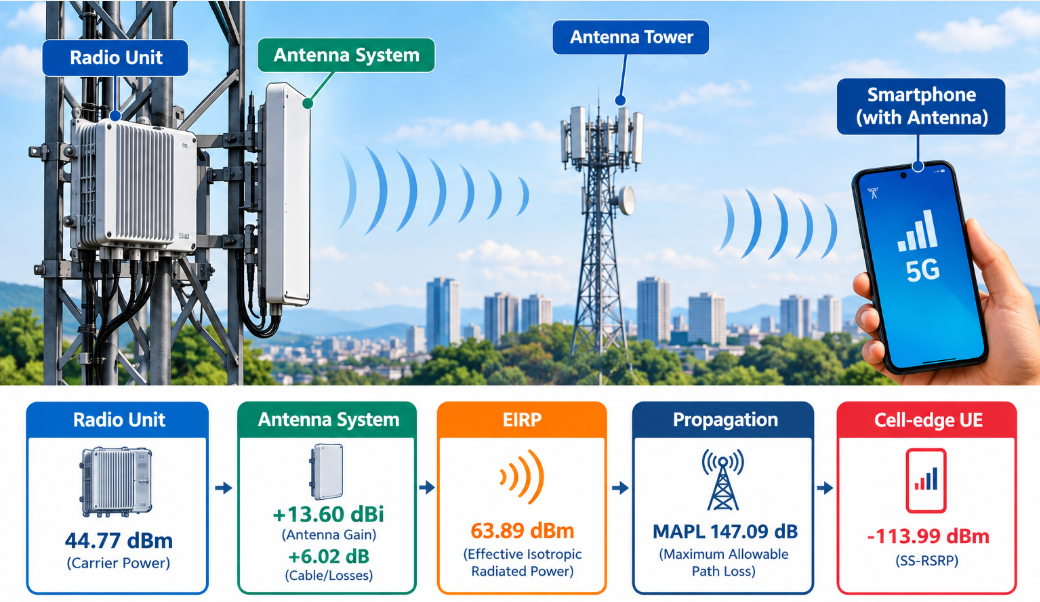
Figure 1. End-to-End Link Budget chain used for the modeled n71 coverage calculation.
Cable Loss = 0.5dB
Model at a glance:
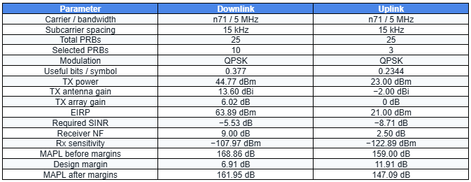
Figure 2. Link Curve Values
n71 • 5 MHz • 15 kHz SCS • 25 PRBs • QPSK • Active PRB’s: 10 DL PRBs / 3 UL PRBs
Key result:
Using the active 10 DL PRB / 3 UL PRB, the model we consider is uplink-limited at
147.09 dB post-margin MAPL and gives a minimum SS‑RSRP of −113.99 dBm.
Executive summary
A 5G NR link budget determines the maximum path loss a network can tolerate while maintaining the target cell-edge performance of 545 kbps in the downlink and 102 kbps in the uplink. By combining transmitter characteristics, antenna gains and losses, receiver sensitivity, SINR requirements, and design margins, it derives the Maximum Allowable Path Loss (MAPL)—the primary metric used to define the network's practical coverage limit.
1. What a link budget really does
Coverage is not determined by transmit power alone. A link budget is a chain of constraints: transmit power becomes radiated power through antenna gain and array gain; the signal then encounters propagation and design losses; finally, the receiver must have enough signal relative to thermal noise, noise figure, and the required SINR.
Transmit power establishes the starting energy available to the radio link.
Antenna gain and array gain increase effective radiated power in the modeled/desired direction.
Receiver sensitivity defines the minimum signal level required for the selected operating condition.
MAPL is the maximum path loss that can be tolerated while maintaining the modeled requirement.
Design margins convert an idealized link budget into a more deployment-oriented coverage threshold.
2. n71 carrier configuration
The model is built around a 5 MHz channel Bandwidth of n71 carrier with 15 kHz subcarrier spacing. The carrier contains 25 physical resource blocks (PRBs). For the calculation considered, 10 DL PRBs and 3 UL PRBs are the active cell-edge allocations. Both links use QPSK, with modulation efficiencies taken from the Figure 2. Link Curve values.
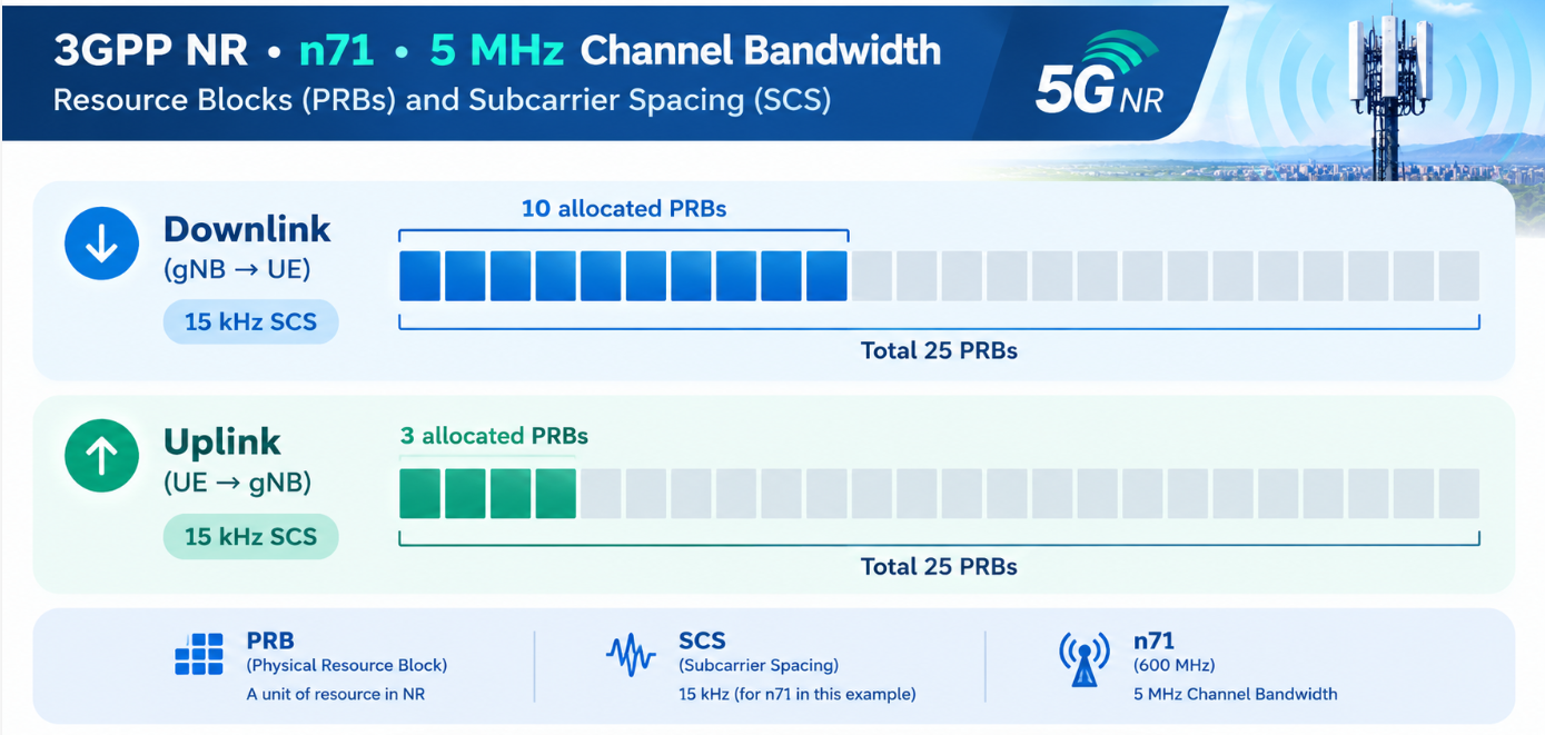
Figure 3. n71 Carrier Active PRB’s used in DL & UL
3. Converting Transmit Power into EIRP
For the downlink, the supplied model starts with 44.77 dBm of Radio Unit power per carrier per physical antenna port. The antenna contributes 13.60 dBi of gain, the 4Tx array contributes 6.02 dB, and feeder/jumper losses discounts/reduces 0.50 dB. The 6.02 dB array gain is 10·log₁₀(4), corresponding to four transmit antennas.
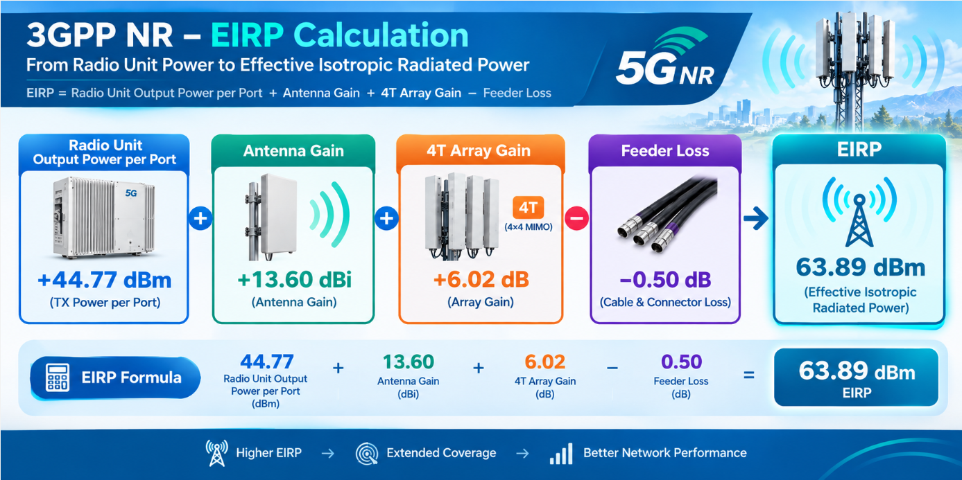
Figure 4. Downlink EIRP Calculation
4. Deriving Subcarrier Reference Power
One NR Physical Resource Block contains 12 subcarriers. With 25 PRBs, the full 5 MHz carrier contains 300 subcarriers. For the SS‑RSRP calculation, the antenna-side downlink power before subcarrier distribution is 57.87 dBm:
Output Power per Antenna port > 44.77 + 13.60 − 0.50 = 57.87 dBm
Dividing this reference power across 12 × 25 = 300 subcarriers gives 24.77 dB of distribution loss. This gets used in the final SS‑RSRP calculation.
Reference Signal Power = 57.87 − 10log10(300)
= 33.10 dBm
5. Receiver sensitivity
Receiver sensitivity is the lowest signal level that enables the receiver to meet the target performance requirements under a given operating condition. To determine it accurately, thermal noise should be computed over the bandwidth occupied by the allocated PRBs for the specific link, rather than across the entire carrier bandwidth.
Formula/Calculation:
Receiver Sensitivity (dBm) = −174 + 10·log₁₀(NPRB × 180,000) + Receiver NF + Required SINR
Noise Figure (NF) is the amount of additional noise introduced by the receiver itself.
The 180kHz term comes from 12 subcarriers per PRB × 15kHz per subcarrier.
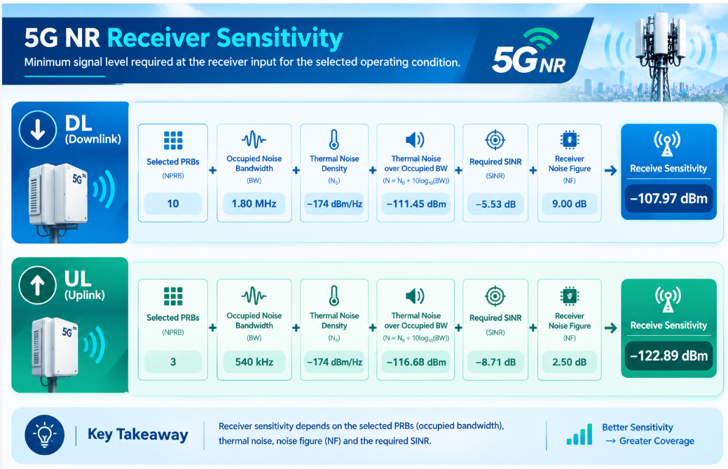
Figure 5. Receiver Sensitivity
6. Coverage Limit Calculation (Calculating MAPL: Integrating EIRP, Sensitivity, and System Gains )
The link budget next combines the transmit-side EIRP with receiver sensitivity, receive antenna gain, diversity/combining gain, RF losses, and other implementation losses. These factors collectively determine the Maximum Allowable Path Loss (MAPL) before the application of coverage, shadow-fading, and other network design margins. MAPL represents the maximum propagation loss the radio link can tolerate while still meeting the target performance requirements. The uplink starts with the lower pre-margin MAPL, so it becomes the limiting direction once the design margins are applied.
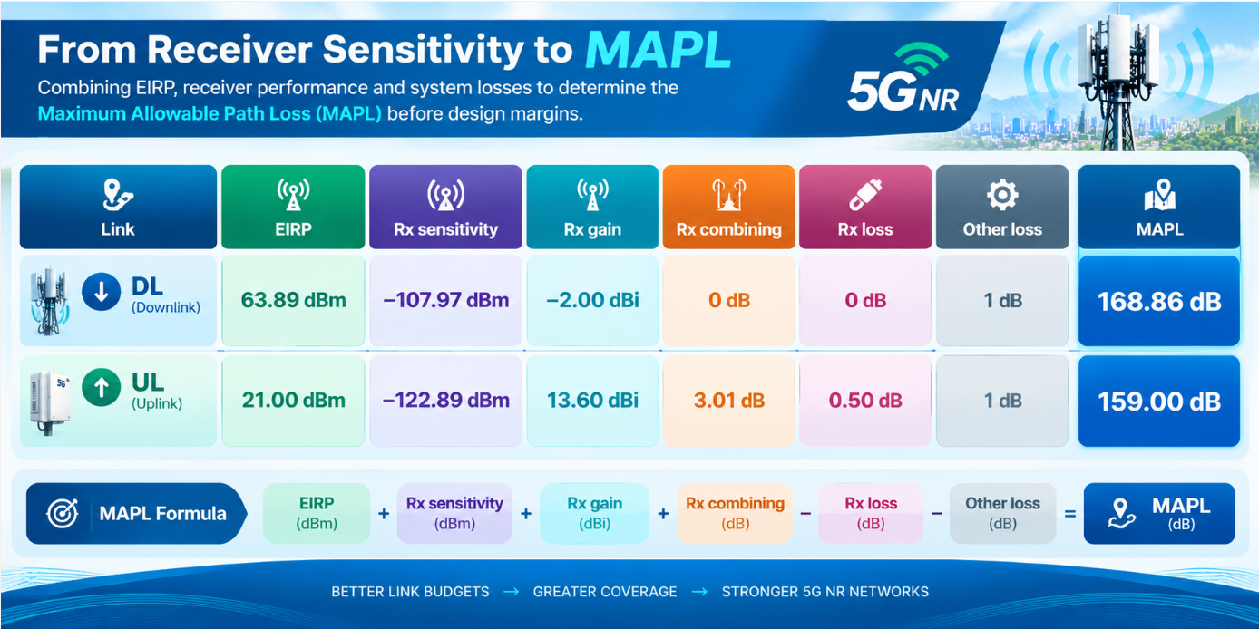
Figure 6. MAPL Derivation pre-Margin Values [Uplink Limited]
7. Applying Design Margins to Derive the Limiting MAPL
The model considered incorporates design allowances for interference, fading, implementation and temperature effects, penetration losses, and other propagation-related factors. An additional other gains term is included to account for expected performance benefits. These values represent engineering assumptions specific to the scenario being modeled and should not be interpreted as fixed or universally applicable constants. Together, these margins adjust the theoretical MAPL to reflect more realistic operating conditions and determine the limiting MAPL used for coverage assessment.
Coverage Constraint: Uplink-Limited Performance
After applying all design margins, the uplink MAPL is reduced to 147.09 dB, compared with 161.95 dB for the downlink. Since the uplink can tolerate less path loss, it becomes the limiting factor for coverage and defines the effective cell radius.
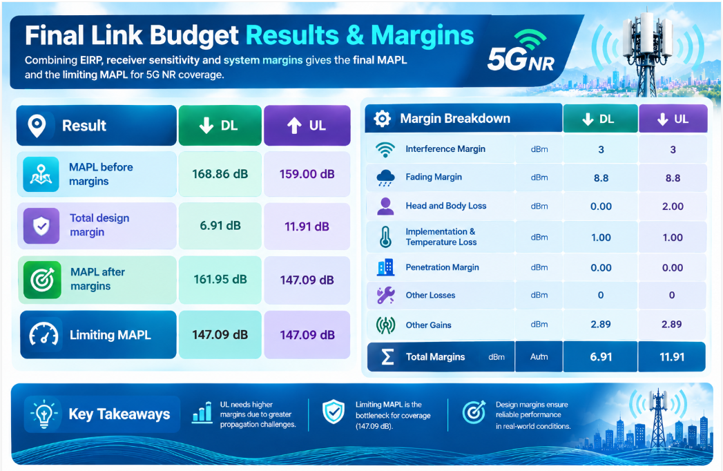
Figure 7. Uplink Design Margin
8. Derivation of the Modelled Cell-Edge SS-RSRP Threshold (Minimum SS‑RSRP at the coverage boundary)
To determine the minimum SS-RSRP at the coverage boundary, the downlink antenna-side power is first allocated across the carrier's 300 subcarriers. The limiting MAPL is then subtracted from the resulting per-subcarrier power level to obtain the minimum signal strength expected at the cell edge.
SS‑RSRP = 57.87 − 10·log₁₀(12 × 25) − 147.09
= 57.87 − 24.77 − 147.09
= −113.99 dBm
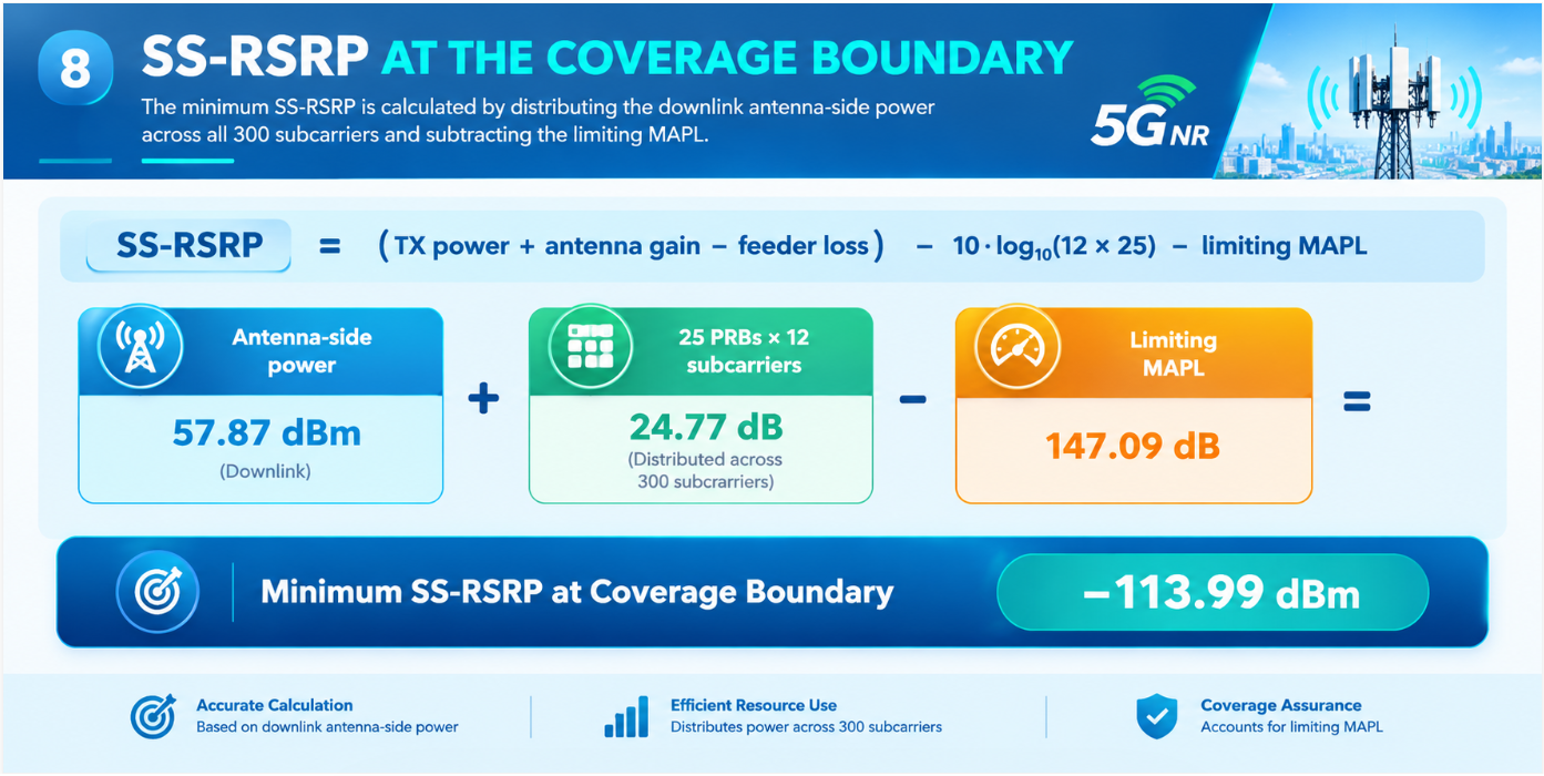
Figure 8. Cell Edge SS RSRP Calculation
9. Key Derivations & takeaways
Low-band n71 can support long-range coverage, however cell-edge performance is governed by the complete link budget rather than EIRP alone.
For a 15 kHz SCS carrier, each PRB represents 12 × 15 kHz = 180 kHz of occupied noise bandwidth.
Receiver sensitivity depends directly on the number of occupied PRBs. Changing PRB allocation changes thermal noise and therefore sensitivity.
In this model, the uplink is the limiting direction after margins, with a 147.09 dB limiting MAPL.
The resulting modeled minimum SS‑RSRP is −113.99 dBm.
Fading, interference, implementation/temperature, and penetration allowances are design assumptions; changing them changes MAPL.
SS‑RSRP must be calculated using one antenna port
Link budgets prevent over‑optimistic coverage predictions
Standards: Per 3GPP TS 38.215 v18.3.0, for FR1, SS-RSRP is measured “at the antenna connector”—i.e., the signal level at a single reception point on the UE.
Regulatory/Standards Guidance: FCC regulations and 3GPP specifications do not require SSB transmission from every gNB antenna port, supporting single-port SS-RSRP modeling for coverage.
Polarization imbalance occurs in practice (e.g., due to device orientation, user grip, or local scattering), especially at the cell edge. As such, the UE may only receive a strong signal from one polarization (antenna port).
At the coverage boundary, environmental effects often mean that only one antenna port’s signal is reliably received above noise/interference levels.
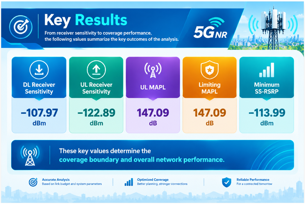
Figure 9. Key Derivations
